Helicopter Navigation – Cross Country Flight Navigation

Redback Aviation Helicopter Flight Navigation

The E6-B Flight Computer

Senior instructor Paul Smith comes to terms with the most important computer pilots use for helicopter navigation

I’VE never liked doing things I don’t fully understand. Why am I doing it and how does it work? Helicopter navigation is an essential part of piloting.

It’s like being a child asking “why?” and copping the parental position of “just do it because I say so”. No-one has ever learned anything that way. Understanding doubles the learning.

Similarly I’ve always found my Flight Computer, an E6-B, to be something of an enigma. It always gives the right answers for course corrections, but I’ve never really understood how. The numerical slide rule face, for me, is relatively straightforward, but not the course correction face. Being a civil engineer, math has always been a reasonably strong point for me.

[easyazon_infoblock align=”right” cloak=”n” identifier=”B004X762EY” locale=”US” localize=”y” nf=”y” tag=”rafsb-20″]

Vector geometry never bothered me either, which is exactly what our Flight Computers are using to give course corrections for helicopter navigation ground speed etc. However, despite being a senior Instructor, I’ve lately been embarrassed to have to admit to Navigation students that I couldn’t properly explain or remember why the damn thing works.

And being reduced to the “parental” response is clearly not a satisfactory training response to my students. So I set out to design my own Flight Computer from first principles, first on graph paper then with scales and protractors Eventually the penny dropped- it finally made sense!

Despite the age of GPS, and because students will always need to do their cross country endorsements from first principles with slide rules, maps, pencils and protractors, there may just be a few others out there in my position too who would benefit from my soul searching. I hope it helps your understanding and improves your safety.

---

Helicopter Navigation: Heading + Wind = Track

When we begin learning to fly, one of our first lessons introduces aeronautical principles around lift and drag and the effect that wind speed relative to the aircraft has on these.

We learn to take off into wind, not downwind, in order to minimize our take-off distance, but once airborne the aircraft is influenced entirely by the wind direction and our relative airspeed, not by any contact with the ground.

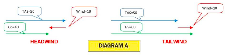
We learn that if the aircraft can lift off at an airspeed (TAS) of 50kts, then a 10kt headwind allows us to be airborne at just a 40kt ground speed (GS). Conversely, a 10kt tailwind means we must achieve a 60kt GS to be airborne.

You have just used (perhaps unwittingly) vector mathematics according to the simple equation.

Heading + Wind = Track where the vectors happen to be parallel and negative (headwind) or additive (tailwind). Diagram A shows the simple vector geometry involved. The vectors have been drawn off-set from each other fore clarity.

What is a vector?

It is a measurement of something which has a directional component to its quantity In our case, the wind vector has direction (degrees true from which it is blowing) and speed (knots).

Its correct term is wind velocity rather than wind speed and is quoted in a standard format such as 270/15. The feature which confuses many students is that the compass bearing quoted with wind speed is MOT the direction TOWARDS which the wind is blowing, but the direction FROM which it is blowing.

This seems counter intuitive because all our other compass bearings for aircraft heading and track are TOWARDS our direction of travel. I suspect the explanation is hidden in the mists of time – we turn our face into the wind to sense its direction because that’s where our sensory organs are concentrated.

We smell smoke from the fire, see rain from the storm, prey smells the hunter coming and vice-versa Hence the direction FROM which the wind is blowing can be a major indicator of potential danger.

Helicopter Navigation: How much can the wind affect heading?

Our other frequent experience of the vector equation above, is having to allow for drift in the circuit to ensure we fly a good rectangular pattern, particularly on the cross-wind and base legs, or when taking off with some cross-wind component and feeling the aircraft “weather vane” into the wind at lift-off.

[easyazon_infoblock align=”right” cloak=”n” identifier=”B003VS6U0M” locale=”US” localize=”y” nf=”y” tag=”rafsb-20″]

Instructions on the flight computer use True Air Speed (TAS). In the past we typically ignored the conversion of IAS (Indicated Air Speed) to TAS because of the low speeds and altitudes at which ultralights flew.

With ultralight aircraft now capable of 125+kts at 10,000ft, we can’t afford to ignore it in many cases. An aircraft flying at 90kts IAS at 5,000ft in 20°C air temperature is achieving 100kts TAS, which is too large a difference to ignore for navigation purposes.

We’ll assume our aircraft flies on a northerly heading at a TAS of 100kts, that the wind speed is 25kts, and that it could be blowing from any direction. Diagram B (approximate scale only) shows all the possible resultant ground tracks and speeds which we can fly under these conditions (green circle). Maximum and minimum GS are 125kts (southerly tail wind) and 75kts (northerly headwind). Several vector samples are illustrated, but two special cases are worth examining.

Example 1:

Northerly heading at 100kts and 25kt westerly wind (270°). The resultant vectors form a right angle triangle where the track speed can be calculated using Pythagoras’ Theorem from simple geometry.

• Track speed2 = Heading speed2 plus Wind speed2

• Track speed2 = 1002 + 252 = 10,625

• Track speed = √10,625 = 103kts

• Track direction = angle which has tangent = 25 ÷ 100 = 0.25,

• hence 14°02′

Example 2:

Maximum deviation from our northerly heading is defined by the resultant track which is tangential to our 25kt wind circle, which is a slightly more easterly result than Example 1. Again this is a right angle triangle but defined slightly differently because the right angle is in a different position.

• Track speed2 = Heading speed2 minus Wind speed2

• Track speed2 = 1002 – 252 = 9,375

• Track speed = √9,375 = 97kts

• Track direction = angle which has sine = 25 ÷ 100 = 0.25,

• hence 14°29′

These two examples demonstrate that in some simple cases where vectors are at right angles, the calculations are relatively straightforward using simple geometry, even if you have to re-read your high school text books. It also explodes the commonly held view by many pilots that the largest deviation from your heading is caused by a wind at right angles to that heading.

In fact, it’s caused by a wind with a slight headwind component the actual bearing of which will vary depending on the ratio of wind speed to your TAS, and in our example blowing from 284° 29′ not from 270°.

The error caused by this incorrect assumption is relatively minor, around half a degree, or 0.5 nautical miles in 60 in our examples. Remember the basic rule of thumb that 1 in 60 approximates one degree? Clearly the error increases for slower aircraft in stronger winds, around 3.5 nautical miles in 60 for a TAS of 60 and wind speed of 30.

Another fallacy commonly expressed by pilots, that a wind directly abeam your heading has no affect on your ground speed, is clearly demonstrated as false – 100 TAS becomes 103GS in Example 1.

In summary then, the maximum possible deviation from our heading for any given wind speed is defined by the angle having its Sine = Wind speed – TAS.

If the reader wants to research the more complete set of equations, Wikipedia has a good article on both the history of the E6-B and the full geometrical equations.

• Sine (Max Deviation Angle) = Wind Speed ÷ TAS

• Max Deviation Angle = Sine-1 (Wind Speed ÷ TAS)

Next: How to apply this to the Flight Computer.

Helicopter Navigation: How much can the wind affect heading?

Our other frequent experience of the vector equation above, is having to allow for drift in the circuit to ensure we fly a good rectangular pattern, particularly on the cross-wind and base legs, or when taking off with some cross-wind component and feeling the aircraft “weather vane” into the wind at lift-off.

Instructions on the flight computer use True Air Speed (TAS). In the past we typically ignored the conversion of IAS (Indicated Air Speed) to TAS because of the low speeds and altitudes at which ultralights.

Helicopter Navigation: Ground Speed?

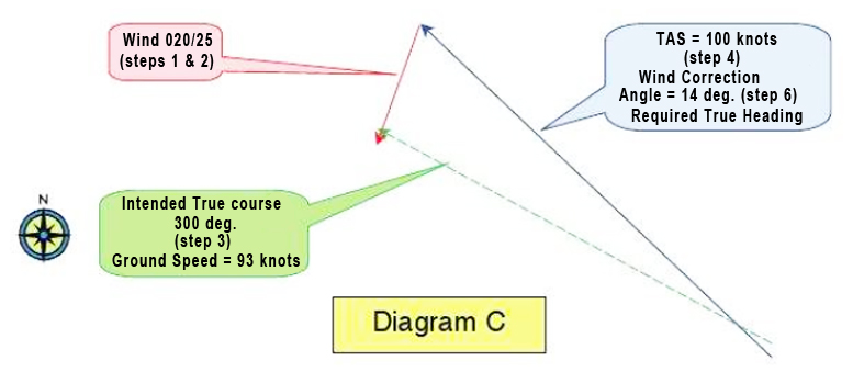
Diagram C represents the final vector geometry to an approximate scale and Diagram D shows how it’s constructed together with portions of the Right Computer’s line – work (arcs of speed circles and radials of headings). The relevant instructions listed on the face of the computer are noted as sequential Steps 1 – 6.

EB6 Flight Computer Instructions

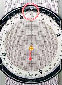
Step 1: Set wind direction under True ◯

Index: Turn compass rose so that 020° shows under the True Index

Step 2: Mark Wind Velocity up torn Center Point. It doesn’t matter where the Center Point (or grommet) is on the graph lines, but normally you would position the grommet on one of the velocity circles to make it easy to measure wind velocity up the center line.

I’ve chosen the 150kt circle, ⊕ so the wind velocity mark will be made at the 175kt position, 25kts up. You have effectively drawn the Wind Vector of 25kts from 020′ to the grommet.

Step 3: Set true Course under True Index. ◯ Turn compass rose till 300° shows under the True Index. As you do this the wind velocity mark rotates to the right. You have now created the course vector(green) intersecting the wind vector (red) at the center point (grommet).

Step 4: Slide Wind Velocity mark to True Airspeed By siding the circular compass section of the computer up or down the inner rectangular section, you can see that the red Wind vector is moving up or down the green True Course vector.

In order to complete the triangular geometry you just move the red Wind vector until the Velocity mark intersects the TAS circle of 100. In our case that is in a downwards direction. If our TAS was 200 then we would move it upwards to that circle.

Step 5: Ground Speed reads under the Center. The GS now can be read under the tip of the red Wind vector where the grommet is, namely 93kts. This makes sense because the wind has a slight headwind component.

Step 6: Wind Correction Angle reads between Center Line and Wind Velocity Mark. The Wind Correction Angle lies between the intended True Course (green vector up the center line), and the Wind Velocity Mark. The angle reads 14° to the right of the center line. ◯

This also makes sense because we come to know instinctively that we need to aim slightly into the wind coming from our right in order to make good our intended course – “laying off the drift”. Consequently our True Heading (blue vector) will be 300° + 14° = 314° in order to track 300° over the ground. This simple sum can also be read off the top compass scale.

Step 7: Convert True Heading to Magnetic Heading by adjusting your Magnetic Variation. This final step isn’t directly listed on your computer as a numbered step other than some – where on its face as an equation.

This is the moment we convert our navigation from paper based True values to compass based Magnetic values for cockpit use during flight. In my local area the magnetic variation is around 8° East so I would subtract this value from 314° and get 306° to use as my compass heading.

Due to turbulence and relatively small compass faces, its highly unlikely you’ll be able to hold a heading any better than ±3° but your calculations should carry through to this point to the nearest degree in any case. Your helicopter navigation technique should always refer from ground to map and back again as you fly, thus confirming your intended track.

Helicopter Navigation: Section – 1 – Summary

You’ll note that the vector diagram overlaid on the computer face is identical in shape to Diagrams C and D but rotated with the course vector up the page. The computer has been ingeniously designed so that the rotating compass face is just like rotating your paper map with your course pointing “up” the page.

The concentric circular lines of TAS values from 30 knots to 260 knots and the radial lines of compass bearings are all centered at a point off the bottom of the computer, and the extent of correction angle is limited left and right of the center line. You’ll notice that the correction angle reduces from as little as 10° near the top of your computer to as much as 40° near the base.

This reflects the ratio of wind speed to TAS increasing in the same direction. Refer back to Diagrams B and D. The device represents a limited window of all the possible speeds and correction angles which cover most flying conditions the average pilot will experience, cleverly superimposed with a rotational compass which allows for any course you may wish to fly Genius!

I trust this article has been as illuminating for you in the reading as it has been for me in the making!

Blue skies, enjoyable flying and may you always find your way safely home!

---

Above, Paul set out to design his own helicopter navigation Flight Computer from first principles, on graph paper then with scales and protractors. He explained that despite the age of GPS, and because students will always need to do their cross country endorsements with slide rules, maps, pencils and protractors, there may just be a few others out there who would benefit as he did torn knowing just how an E6B works.

Who Invented The E-B6 Flight Computer?

According to Wikipedia, the E-6B was developed in the US by Naval Lt. Philip Dalton in the late 1930s. Dalton didn’t name it, though. That was the US Army Air Corps in World War 2 which merely gave it an official “part number”, but that’s what its been called ever since. Dalton was a university graduate who signed up for the war as an artillery officer, then became a Naval Reserve pilot.

He was killed with a student in 1941 while practicing spins. He invented and marketed a number of flight computers, including the 1933 Model B. which showed True Air Speed (TAS) and Altitude corrections. Three years later he put a double-drift diagram on the back to create the E-1, E-1A and E-1B flight computers.

In 1937, Dalton added a simple wind slide to his Model B circular slide rule which the Army called the E-6A. A year later, it asked him to make some more small changes, which then became the E6B in 1940. Hundreds of thousands of the devices were made and distributed during the war. Hundreds of thousands more have been sold since.

Helicopter Navigation: Apply the weather to the Flight Computer

In part 1 (above), we calculated what the wind does to our heading, but that’s not how we navigate to our destination. We actually start with our desired track and have to work backwards knowing our forecast wind velocity (speed and direction) to determine on which heading to aim the aircraft.

Note that everything on the computer is expressed in Degrees True, not Magnetic, so we’ll do all the helicopter navigation calculations using our True bearings measured off the paper maps (WAC, VNC or VTC) then apply the magnetic variation as the final step. Some text books suggest applying the magnetic variation to both your intended track and to the wind direction before using the computer, but I believe there are four very good reasons not to start this way for helicopter navigation cross country.

1. All the instructions on the computer are expressed in True terms, which is confusing if you have converted everything to Magnetic first – you could mix up your values quite easy. I know I have done. Embarrassing on your navigational test fights with the instructor!

2. You have to add (West) or subtract (East) magnetic variations twice, to both Wind and to Track, instead of just once to your final True Heading – double the room for errors here.

3. It seems more logical to apply the Magnetic Variation to your calculated True Heading at the end of the process because that’s when you move your thought process from tabletop paper and pencil to the reality of the cockpit, namely your compass.

4. Most importantly the answer is the same because the geometry is the same.

There are other computer designs out there, and at least one other iterative technique for the E6-B described in some texts, but the instructions printed on its face are the most straight forward, especially once you understand what it’s constructing for you. Lets follow the instructions on the top of the computer and relate each step to Diagrams C and D.

Helicopter Navigation: For Ground Speed and True Heading

Example 3:

Wind Direction/Speed = 020°/25kts, Intended Course (Track) =300′, IAS =100kts.

What is our required True Heading and resultant Ground Speed?

Diagram C represents the final vector geometry to an approximate scale and Diagram D shows how it’s constructed together with portions of the Right Computer’s line – work (arcs of speed circles and radials of headings). The relevant instructions listed on the face of the computer are noted as sequential.

Steps 1 – 6. EB6 Computer Instructions

Step 1: Set wind direction under True.

Index: Turn compass rose so that 020° shows under the True Index

Step 2: Mark Wind Velocity up torn Center Point. It doesn’t matter where the Center Point (or grommet) is on the graph fines, but normally you would position the grommet on one of the velocity circles to make it easy to measure wind velocity up the center line. I’ve chosen the 150kt circle, so the wind velocity mark will be made at the 175kt position, 25kts up. You have effectively drawn the Wind Vector of 25kts from 020° to the grommet.

Step 3: Set true Course under True Index. Turn compass rose till 300° shows under the True Index. As you do this the wind velocity mark rotates to the right. You have now created the course vector (green) intersecting the wind vector (red) at the center point (grommet).

Step 4: Slide Wind Velocity mark to True Airspeed. By sliding the circular compass section of the computer up or down the inner rectangular section, you can see that the red Wind vector is moving up or down the green True Course vector.

In order to complete the triangular geometry you just move the red Wind vector until the Velocity mark intersects the TAS circle of 100. In our case that is in a downwards direction. If our TAS was 200 then we would move it upwards to that circle.

Step 5: Ground Speed reads under the Center. The GS now can be read under the tip of the red Wind vector where the grommet is, namely 93kts. This makes sense because the wind has a slight head wind component.

Step 6: Wind Correction Angle reads between Center Line and Wind Velocity Mark. The Wind Correction Angle lies between the intended True Course (green vector up the center line), and the Wind Velocity Mark The angle reads 14° to the right of the center line.

This also makes sense because we come to know instinctively that we need to aim slightly into the wind coming from our right in order to make good our intended course – “laying off the drift”. Consequently our True Heading (blue vector) will be 300° + 14° = 314° in order to track 300° over the ground. This simple sum can also be read off the top compass scale.

Step 7: Convert True Heading to Magnetic Heading by adjusting for Magnetic Variation. This final step isn’t directly listed on your computer as a numbered step other than some – where on its face as an equation.

This is the moment we convert our helicopter navigation from paper based True values to compass based Magnetic values for cockpit use during flight. In my local area the magnetic variation is around 8° East so I would subtract this value from 314° and get 306° to use as my compass heading.

Due to turbulence and relatively small compass faces, it’s highly unlikely you’ll be able to hold a heading any better than ±3° but your calculations should carry through to this point to the nearest degree in any case. Your navigation technique should always refer from ground to map and back again as you fly, thus confirming your intended track.

Helicopter Navigation: Section – 2 – Summary

You’ll note that the vector diagram overlaid on the computer face is identical in shape to Diagrams C and D but rotated with the course vector up the page. The computer has been ingeniously designed so that the rotating compass face is just like rotating your paper map with your course pointing up the page.

The concentric circular lines of TAS values from 30 knots to 260 knots and the radial lines of compass bearings are all centered at a point off the bottom of the computer, and the extent of correction angle is limited left and right of the center line. You’ll notice that the correction angle reduces from as little as 10° near the top of your computer to as much as 40° near the base.

This reflects the ratio of wind speed to TAS increasing in the same direction. Refer back to Diagrams B and D. The device represents a limited window of an the possible speeds and correction angles which cover most flying conditions the average pilot will experience, cleverly superimposed with a rotational compass which allows for any course you may wish to fly Genius!

I trust this article has been as illuminating for you as the reading as it has been for me in the making! Blue skies, enjoyable flying and may you always find your way safely home!

---

COURTESY: Recreational Aviation Australia Sport Pilot Magazine

---

VIDEO: Private Pilot Airplane – Navigation – ASA (Aviation Supplies & Academics)

---

VIDEO: How Pilots Know Where To Go – Using A Plotter